Avoiding Pitfalls in Calibrating a Water Distribution System Model
Tom Walski, Ph.D., P.E., F. EWRI1
Bentley Systems, 3 Brian’s Place, Nanticoke, PA 18634, tom.walski@bentley.com
ABSTRACT
For a model to have credibility, it needs to be calibrated against data from the distribution system. While this sounds simple, there are issues that can steer the calibration in the wrong direction. This paper discusses some common pitfalls and how to avoid them.
INTRODUCTION
Water distribution model calibration is easy. The modeler just builds the model; measures a few pressures; compares them with the model; if they don’t quite agree, adjusts some C-factors; and declares the model calibrated. Those steps may yield a model that can be useful for some purposes but there will be many situations where that model will be inaccurate to the point where it is misleading.
There are really two steps to making adjustments in order to resolve discrepancies between the model and field data:
- Determine WHY there is a discrepancy
- Correct the discrepancy
Roughly 90% of the effort in model calibration is involved with the first step. Once the source of the discrepancy is determined, it’s usually fairly easy to make the adjustments. However, the research literature on model calibration (AWWA Calibration Subcommittee, 2013b) has focused almost exclusively on the second step. Without successfully completing the first step, the second step involves making an assumption (often a wild guess) about the source of the discrepancy and adjusting that parameter or questioning field data. For example, a common guess is to assume that the present roughness values are wrong, however, without validating the assumption with the age of the pipes and performing some empirical analysis beforehand to check if a relationship between the age and roughness can be developed.
An overview of model calibration is provided by the AWWA Calibration Subcommittee (2013a). While there have been a large number of case study and research papers on model calibration (AWWA Calibration Subcommittee, 2013b), there are not many documents on the practical aspects of model calibration (AWWA, 2017; Hirrel, 2008; Ormsbee and Lingireddy, 1997; Speight, et al., 2010; Walski, 2010).
The assumption as to the source of the discrepancy is frequently incorrect because there are so many sources of the problem. Table 1 gives a partial list of the sources of discrepancies.
Approaches based on automated calibration or parameter estimation are incapable of arriving at a good solution when there are so many sources. Usually, the modeler will assume that the error is due to incorrect pipeline as roughness (usually C-factor) or demand placement/multiplier factors and adjust those parameters accordingly. Walski (1983) wrote one of the earliest papers on this type of approach. It wasn’t long that he realized that this type of approach wasn’t necessarily correct (Walski, 1986). Adjusting the wrong parameter could result in better calibration but this may be due to “calibration by compensating errors” (Walski, 1986). An error in one input could often mask an error in another input.
Table 1. Calibration Sources of Error
| Inaccurate pipe roughness |
| Inaccurately placed demands |
| Inaccurate demand magnitude |
| Incorrect demand patterns |
| Incorrectly closed valves |
| Incorrect model connectivity |
| Incorrect elevation data |
| Inaccurate pressure and flow sensors |
| Wrong pump curves |
| Wrong pump operating status/speed |
| Wrong tank/reservoir water levels |
| Wrong control valve (e.g. PRV) settings |
| Adjusting base demand with data not collected in base period |
| Incorrect pressure zone boundaries |
| Incorrect pipe size/age/material in GIS/maps |
| Unknown pipe restrictions |
| Incorrect water quality reaction rates |
| Failure to reach steady pressure conditions due to transients |
| Atypical demands (e.g. special events) not accounted for when measuring pressure |
| Uncertainty whether SCADA pressure/flow readings were instantaneous or temporally averaged |
| Changes made to system since model built |
| Values from “latched” sensors in SCADA |
When faced with a complex extended period simulation (EPS), there are more parameters to adjust than most modelers can handle. Instead of trying to adjust everything at once (and become confused) or assume the source of errors in known a priori (often a bad assumption), it is preferable to use different types of data for what is best starting with the simplest data to adjust the simplest parameters and moving on to more complex adjustments (Walski, 2017). The types of data and the adjustment they support are summarized in Table 2.
Table 2. Types of Data and How They Can Be Best Used
| Type of Data | Adjustments
|
| Steady state, normal demand | Pressure zone boundaries, pump curves, PRV settings
|
Steady state, high flow
| Pipe roughness, demands, closed valves, connectivity
|
EPS, controls known
| Demand patterns
|
EPS, controlled by control statements
| Pump and valve controls
|
The key to this approach is to realize that during a normal day, the hydraulic grade is relatively flat such that models are relatively insensitive to parameters like pipe roughness or closed valves. It is only when the velocity and head loss increase, due to peak demands or fire hydrant flows, that the discrepancies caused by these parameters can be detected. The benefit of this type of step-by-step calibration is that once a set of adjustments are made, it is unlikely that the modeler will need to go back and change parameters (although there may be exceptions). The step-by-step investigation and independent calibration can be achieved via first creating a base scenario and then building upon it by modifying suitable physical parameters based on the specific scenario or error source. By doing so, a series of scenarios is developed which allows for easy tracking and validation in the later model testing phase.
An important concept to remember is mathematician George Box’s (1976) famous quote, “All models are wrong, some are useful”. “Useful” is what hydraulic modelers should be targeting.
The following section provide some examples where calibration could have been done batter.
DATA ACCURACY
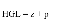
Comparisons between the model and field data are best made in hydraulic grade units. With such data, it is easy to spot outliers such as an inaccurate gauge and an assumption that the elevation of the model node is the same as the elevation of the pressure gauge (an assumption often assumed away in research papers). The hydraulic grade is given by
 (1)
(1)
Where HGL is hydraulic grade line, L; z is the elevation of the pressure gauge, L; p is the pressure head, L
Even if the modeler has a pressure gauge with accuracy of 0.1 m, which is seldom true in the field, if the elevation data is accurate to 5 m, the HGL is accurate to +/- 5 m.
The availability of pressure data from SCADA (Supervisory control and Data Acquisition) system and IIOT (Industrial Internet of Things) often present data with ridiculous precision. It is not uncommon to see such data reported as pressure = 65.785401 m even though the real value 66 +/- 2.
The problem is further exacerbated by small transient waves that bounce around most water distribution systems. Even if the true reading is 65.78 m, the pressure gauge at any point in time can read 66.17, 63.98, 65.4, … It is important to understand what the values from the SCADA system mean. Are they instantaneous readings at the time of the polling interval or are they average valves during the previous polling interval? Average values are usually preferred as they should be closer to the true value.
Often, the elevation of the pressure gauge is not known. It may be necessary to use a GPS to determine the elevation or if the node elevation is taken from a digital elevation model, an adjustment can be visual. It may be helpful to take photos of the model node and of the pressure gauge for error checking.
RANGE OF CALIBRATION CONDITIONS
Most calibration data are collected on normal days. (That’s what makes them normal.) As mentioned above, the hydraulic grade is relatively flat, which means that results are not very sensitive to pipe roughness and demands. This enables the modeler to focus on getting the boundary conditions right. However, some modelers try to use this data to adjust pipe roughness. There are several problems with that approach. The problem with data accuracy is covered in the previous section.
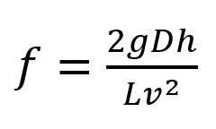
A bigger problem is that in order to have confidence in pipe roughness calculations, it is necessary to have head loss an order of magnitude greater that the error in measurement. These calculations (in the case of the Darcy-Weisbach equation) boil down to
(2)
Where f = friction factor; g = gravitational constant, L/T2; D = diameter, L; h = head loss, L; L = pipe length, L; v = velocity, L/T.
While g, D, and L can be known with some accuracy, v is close to zero and h is not only close to zero but has a large uncertainty. This means that equation (2) is essentially
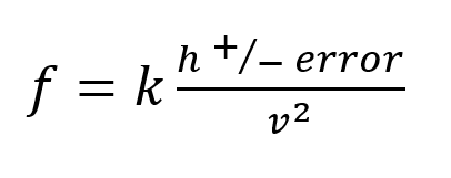 (3)
(3)
Where k =2gD/L
In many systems, especially in North America, pipes are sized conservatively such that eh error in measurement of h is often on the same order of magnitude as h.
The implication here is that the modeler may have 10,000 pressure readings from a SCADA sensor, but for model calibration, they are useless other than to ensure the boundary conditions and elevation data are not grossly in error (Walski, 2000).
This problem can be overcome in several ways. For large transmission mains, the velocities can be meaningful, and the length of the test section can be sufficiently large such that h and v are significant. For distribution system piping, it is often necessary to conduct a hydrant flow test to reach sufficient head loss to determine roughness or locate closed valves.
USING A SINGLE SCENARIO
If the only data available to check calibration is collected during normal days, the modeler and other users can feel comfortable using the model on normal days. But that is only one the reason models are built. They are also built to simulate those days when different scenarios arise—fires, pipe breaks, shutdowns, unusual peak demands, i.e. anomaly events.
To have confidence that the model will work well when the system is under stressed conditions, it is essential to collect some field data when the system is stressed. This can be simulated using a standard fire hydrant flow test with a little additional data. It is very helpful to know the boundary conditions for the model which would include which pumps are running, what the water level is in any tank and water the control valve settings are. Errors that are undetectable at low flow can become obvious at high flow as shown in Figure 1.
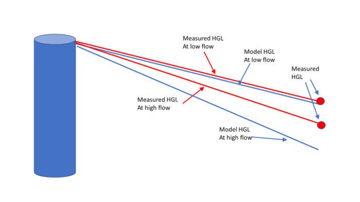
Figure 1. Discrepancies that are hidden at low flow become obvious at high flow
An engineer doing a study on river flooding will not have a lot of confidence in a river model that was calibrated during a drought. Similarly, it is not easy to have confidence in a water distribution system model that was only calibrated for a single condition.
ASSUME SOURCE OF DISCREPANCIES IS KNOWN
Another common issue with calibration, especially in research papers, is the assumption that all discrepancies are due to pipe roughness. This goes back to the earliest research studies (Eggener and Polkowski, 1976). At first, this seem reasonable since it is not feasible to see inside pipes. This carries with it the unreasonable assumption, however, that the model is otherwise perfect, which is highly unlikely. Table 1 is evidence of that.
Adjusting roughness is most important when dealing with system with old, unlined cast iron pipes as roughness can vary widely for that material (Sharp and Walski, 1988). Newer pipe materials do not lose carrying capacity as fast and those old pipes are gradually being removed from system, making roughness adjustments less important as time goes on.
Adjusting roughness, however, can provide insights. If a C-factor of 170 is required to get acceptable results, the implication is that the model does not have sufficient carrying capacity. This can be due to an error in connectivity where an important connection is needed but since that connection is missing, other pipes must carry excessive flow. Figure 2 shows the type of problem that may exist in the underlying network connectivity. A C-factor of 15 would indicate that the system has much less carrying capacity that the model. This could indicate incorrectly closed isolation valves in the system. Conversely, the need to increase demands to an unreasonable level could indicate a large undetected leak or a closed valve as shown in Figure 3. Figure 4 shows how an incorrect roughness can be used to compensate for an incorrect tank water level.
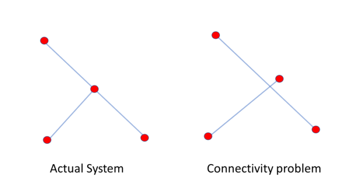
Figure 2. Connectivity issue needs to be corrected, not by adjusting roughness
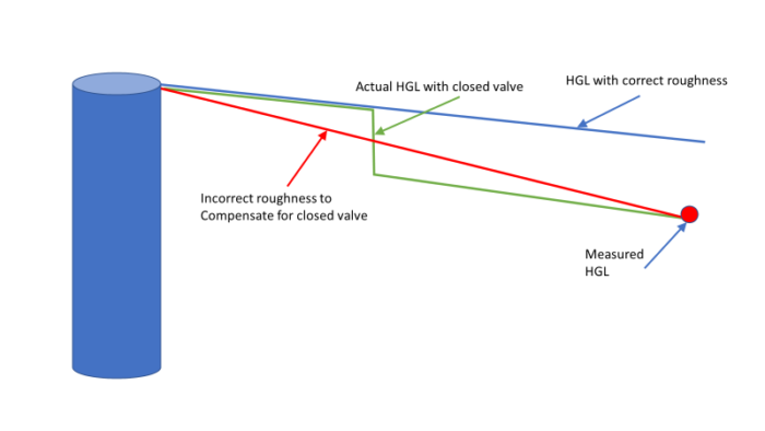
Figure 3. Using incorrect roughness to compensate for closed (or partly closed) valve
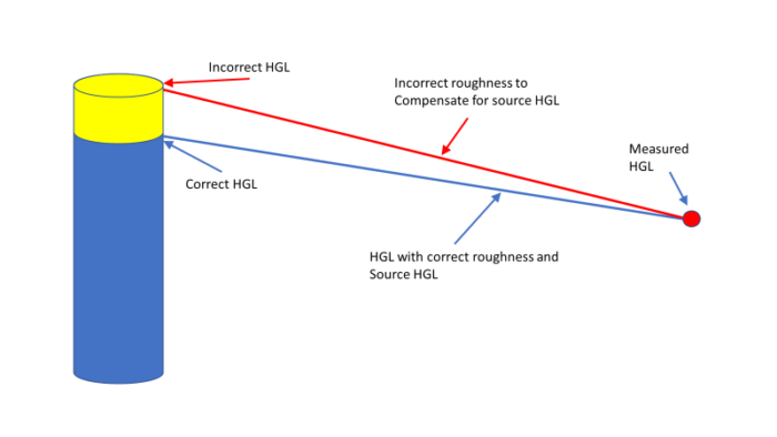
Figure 4. Using incorrect roughness to compensate for incorrect boundary HGL
Such questionable values would indicate that the modeler needs to do the detective work to understand the source of the discrepancy (Walski, 1990).
USING FLOW CONTROL VALVES TO CONCEAL PROBLEMS
Actual flow control valves (FCV), which limit flow in a pipe, are very rare in water distribution systems. Nevertheless, some models have FCVs that don’t exist in the real system. This is often a desperate attempt to match model flows to measured flows. This can make the model appear calibrated for a small number of data sets. However, when the model is applied to new situations, such as addition of a new pump upstream, this can lead to misleading results.
A similar quick fix is to use an inflow (i.e. negative demand) to force a flow reading. This can work in the short run where there is a single pump and the resulting pump head corresponds to a point on the pump’s head characteristic curve. This can be misleading if there are multiple pumps, demands change in different scenarios or the resulting head is not on the pump curve.
Once again, a better solution is for the modeler to understand why the flows in the model do not match the field data.
MAKING ASSUMPTIONS INSTEAD OF GETTING ANSWERS
Sometimes anomalous events (e.g. fire, pipe breaks, special events, shutdowns) will occur in distribution systems. The data collected during that event may not be useful or may shed some light on system behavior. The tendency is to assume away these events or use unrealistic values to account for it. The modeler should communicate with the system operators to determine what exactly happened.
An important facet in model calibration is regular communication between the modeler and system operators. It is much better to resolve issues with a quick phone call or email when they are first detected than to submit a report based on a bad assumption. Talk to the operators.
SUMMARY
This paper pointed out some common mistakes made in model calibration with the hope that novice modelers (and even many experienced modelers) will not fall into them.
ACKNOWLEDGMENT
Review comments on the first draft were provided by Dr. Alvin Chew from Bentley Systems.
REFERENCES
AWWA, 2017 (4th ed.). Computer Modeling of Water Distribution Systems. AWWA, Denver.
AWWA Model Calibration Subcommittee, 2013a, “Defining Model Calibration,” Journal AWWA, Vol. 105, No. 7, p. 60, Denver.
AWWA Model Calibration Subcommittee, 2013b, “Hydraulic Model Calibration: What Don’t We Know,” AWWA Distribution System Symposium, Denver.
Box, G., 1976, “Science and statistics”, Journal of the American Statistical Association, 71 (356): 791–799, doi:10.1080/01621459.1976.10480949.
Eggener, C. and Polkowski, L., 1976, “Network Models and the Impact of Modeling Assumptions,” Journal AWWA, Vol. 68, No. 4, p. 189.
Hirrel, T.D., 2008. How Not to Calibrate a Hydraulic Network Model. Journal AWWA, 100:8:70.
Ormsbee, L. & Lingireddy, S., 1997. Calibrating Hydraulic Network Models. Journal AWWA, 89:2:42.
Sharp, W. and Walski, T., 1988, “Predicting Roughness in Unlined Metal Pipes,” Journal AWWA, Vol. 80, No. 11, p. 34, November.
Speight, V.; Khanal, N.; Savic, D.; Kapelan, Z.; Jonkergouw, P.; & Agbodo, M., 2010. Guidelines for Developing, Calibrating and Using Hydraulic Models. Water Research Foundation, Denver. www.waterrf.org/
Walski, T., 1983 “A Technique for Calibrating Water Network Models,” Journal Water Resources Planning and Management, Vol. 109, No. 4, p. 360, October.
Walski, T., 1986, “Case Study: Pipe Network Model Calibration,” Journal of Water Resources Planning and Management, Vol. 112, No. 2, p. 238, April.
Walski, T. 1990, “Sherlock Holmes Meets Hardy Cross, or Model Calibration in Austin, Texas,” Journal AWWA, Vol. 82, No. 3, p. 34, March.
Walski, T., 2000, “Model Calibration Data: The good, the bad and the useless,” Journal AWWA, Vol. 92, No. 1, p. 94, January.
Walski, T.M., 2010. Practical Tips on Work Flows for Modeling. 2010 AWWA Distribution System Symposium, Denver.
Walski, T., 2017, “Procedure for Hydraulic Model Calibration,” Journal AWWA, Vol. 109, No. 6, p. 55, June.
If you want to look up past blogs, go to https://blog.bentley.com/category/hydraulics-and-hydrology/. And if you want to contact me (Tom), you can email tom.walski@bentley.com.
Want to learn more from our resident water and wastewater expert? Join the Dr. Tom Walski Newsletter today!