
Readers of this blog already know the basics of how to calibrate a water distribution system model. Compare system data with model results and make the necessary adjustments so that the model agrees with the data. But not all data are equal. Some data are valuable; others are of poor quality and must be discarded, while other data looks good but is useless. How to tell the difference?
Understand why data is being used
It’s important to understand why data is being used. If data is used to evaluate the model when head loss is very low, then that data cannot shed any insights regarding pipe roughness, demands, or closed valves. To make those adjustments in anything that affects head loss, there must be measurable, meaningful head loss. Unfortunately, in most developed countries, especially North America, velocity in pipes under normal conditions are low and head loss is therefore often minimal. It is often on the same order of magnitude as the error in measurements. To make any adjustments to pipe roughness, or similar input (e.g. closed valves), it is necessary to have significant head loss. For example, calculating C-factor essentially boils down toC = k V/h0.54
Where V = velocity, h = head loss from source, k reflects system and unit conversions. If measurement of V and h are essentially small number +/- an error value on the same order of magnitude, then C is essentially 0/0. In many cases, velocity and head loss are low during normal demands. Therefore, such data is useless for roughness calculations. In these models, large changes in C have only a small impact on the hydraulic grade line when head loss is low.Accuracy of the field data
The accuracy of the field data depends on the accuracy of both the pressure gauge and the elevation of that gauge. The pressure gauge may be accurate to +/- 1 psi (2.3 ft) but if the elevation of the gauge (not the model node) is only accurate to +/- 5 ft, then the hydraulic grade is only accurate to about 7 ft. If the head loss is 10 ft, the head loss is 10 +/-7. It is difficult to calculate accurate C-factors. Data collected when head loss is low can be useful for such things as checking that pressure zone boundaries and boundary conditions (tank water level, PRV settings), and pump curves are correct. Adjustments to these values, if necessary, should be performed prior to moving on to more hydraulically demanding calibration. But this is just a prelude to the more difficult steps when head loss becomes significant. With large transmission mains, the velocity can be sufficiently high, and the lengths sufficiently long to produce significant head loss. For smaller distribution mains, it is usually necessary to conduct hydrant flow tests to get sufficient head loss to get a meaningful comparison between the measured and modeled HGL values.Calibration of models
I am amazed when someone says their model is calibrated but have only used data collected during low flows. This “calibration” means that there are no gross errors in the model. However, the model user can only have confidence in model results for the range of conditions corresponding to the calibration data. The crucial times for model use are usually peak days, fire flows, shutdowns when flow patterns change and other high flow situations. Even without high flow calibration, the model may be producing good results for these high flow conditions, but users can have more confidence in the results if the model was calibrated for a wide range of flow. Suppose someone calibrated a river flow model during a drought. Would they have much confidence in using that model during a flood? Same can be said for a model to be used for fire flow analysis that was only calibrated for average day flows. In a water distribution system, an incorrectly closed valve or a very tuberculated section of pipes will not be detected during low flow conditions because the velocity and head loss are so low. The confidence that a modeler has in the model is enhanced with the range of conditions for which the model was calibrated. If the model agrees with the field data for both high and low flow conditions, the modeler can have confidence with flow conditions in between. To get more in depth information on this topic see:Walski, T., 2000. “Model Calibration Data: The good, the bad and the useless,” Journal AWWA, Vol. 92, No. 1, p. 94, January.
And if you want to contact me (Tom), you can email tom.walski@bentley.comWant to learn more from our resident water and wastewater expert? Join the Dr. Tom Walski Newsletter today!