In the first part of this blog series, we saw some tips on how to find the solvers that would be best suited to help you in your challenges and studies for stormwater systems. This blog will continue to explore this topic but will focus on sewage and combined systems. 

Reduce Time and Prevent Errors in Wastewater Networks

A wastewater network’s main objective is to collect and convey sewage to a sewage treatment plant (STP) and avoid dumping it into rivers and the environment without treatment. Even though some variation is expected to be observed in the wastewater's flow and load, sudden changes in this pattern can impact the efficiency of the treatment processes.

For example, inflow and infiltration (I&I) high peaks during wet weather periods could exceed the capacity of the collection system or the treatment plant. This results in untreated wastewater in the environment. In this instance, RTK for Rainfall Derived Infiltration and Inflow is important to calibrate the sanitary system hydraulic model. OpenFlows SewerGEMS can help your team to assess this sort of problem and develop solutions.

With this unique, versatile, and powerful solution for sewage, drainage, and combined networks, engineers and sanitary network designers can reduce time and error in their projects. OpenFlows SewerGEMS will enable you and your team to accelerate your projects to the next level with constraint-based design routines, advanced scenario management, easy-to-use graphic user interface (GUI), easy-to-build and easy-to-maintain tools to keep your hydraulic model accurate, and updates that will save time and effort in decision-making. 

Powerful solution for sewage, drainage, and combined networks.

OpenFlows SewerGEMS enables you and your team to accelerate your projects with constraint-based design routines and advanced scenario management. The intuitive graphical user interface (GUI) combined with the easy-to-build and easy-to-maintain tools to keep your hydraulic model accurate and up-to-date allows you to save time and effort for critical decision-making.

SewerGems for Engineers and Sanitary Network Designers.

Beyond these advantages of the software, OpenFlows SewerGEMS also integrates seamlessly with the most popular CAD and GIS platforms (MicroStation, ArcGIS Pro, ArcMap, and AutoCAD). You choose whether you want to run OpenFlows SewerGEMS as a standalone platform or run it within the other platforms. Running OpenFlows SewerGEMS as a standalone platform eliminates the need for an additional subscription to another software. If you choose to integrate OpenFlows SewerGEMS into one of the compatible platforms, you can improve the design, management, publishing, and sharing of 2D and 3D drawings, BIM data, geographic maps, and models.

5-in-1 solution for every type of Sanitary Network 

Wastewater, stormwater, and combined collection systems rely on complex pumping systems and gravity pipes that are partially full or dry. That complexity is reflected in the hydraulic conditions; therefore, calculating the hydraulic behavior is difficult without the right tools.

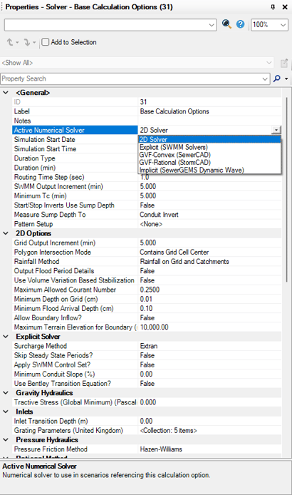
To solve these problems, OpenFlows SewerGEMS has 5 solvers: GVF-Rational, GVF-Convex, Implicit Dynamic, Explicit Dynamic (SWMM) and 2D solver. Each one was designed to help you with different conditions and challenges. 

"From pressure to gravity pipes, from stormwater to wastewater, and from simple to complex systems, your team won´t need anything else." 

This difficulty is exactly why OpenFlows SewerGEMS offers a huge advantage to the user! OpenFlows SewerGEMS has four solvers: GVF-Rational, GVF-Convex, Implicit Dynamic, and Explicit Dynamic (SWMM). Each one was designed to help you with different conditions and challenges.

It empowers users to find and choose the best solution for each scenario and situation! Different solvers will help you adapt to every sanitary network and hydraulic behavior without switching between other software and converting files.

How do I choose the right solver for my sewer or combined sewer network?

If you are scratching your head trying to figure out which solvers will give the answers you're looking for, you should ask yourself these questions about the network you are working on:

• Does this network only convey wastewater, or is it a combined system? 
• Is the flow steady or unsteady?  
• Do I have normal depth conditions in the pipes, or are there also surcharge flow and overflow in the manholes?  
• How complex is the pumping system?  
• Are there loops?  
• Do I have pressure pipes or is your system only gravity pipes?  

To design for sanitary systems operation (combined and sewer), the solver options would be either the GVF-Convex or the dynamic solvers (Explicit and Implicit). I wouldn't recommend the GVF-Rational for a combined system. Although you could use the Modified Rational method with multiple catchments using differing Times of Concentration and entering fixed inflows at nodes to represent sanitary loads, only one critical storm duration is entered.

It is recommended to use the GVF convex solver when working with sanitary networks without significant wet weather flow and designed not to overflow, and systems that consist of primarily force mains or pressure sewers. The Implicit and Explicit solver should be used if you are working with combined systems to study LID best practices or to control overflows in systems with combined inflows or excessive I&I. 

Implicit Solver

The implicit solver uses a four-point implicit finite difference solver to find the numerical solutions for the hydrodynamic Saint-Venant equations. This method was developed by Bentley, based on the US National Weather Service FLDWAV model, to account for conditions in collection systems such as drop manholes and transition between gravity and pressure flow.

It simultaneously solves for both flow and hydraulic grade and uses the same equations for gravity and pressure portions of the system. The implicit solver only solves dynamic flows (not steady state), and the manhole initial elevation is not considered, so the initial manhole elevation is assumed to be the same as the downstream start elevation. Another aspect is that it interpolates flows between the final flow in the hydrograph and the end time. 

The implicit solver tends to be more stable with pumping situations and perform better than the explicit with short pipes and loops in the network. 

Explicit (SWMM) Solver

As the name states, the explicit solver solves the full Saint-Venant equations using an explicit numerical method based on the EPA Stormwater Management Model version 5 (SWMM). It also simultaneously solves for both flow and hydraulic grade and uses the same equations for gravity and pressure portions of the system.  

Besides the Saint-Venant Dynamic Wave and Diffusive Wave (ignoring the Dynamic Wave inertial term) solutions, it can also route flows using further simplification. Examples of these simplifications are the kinematic wave solution and a uniform flow solution, which cannot account for backwater effects.  

The simplifications are achieved by eliminating terms of the dynamic equation, which results in benefits for the models such as simpler formulation, more accessible programming codes, and increased computational efficiency. 

The explicit solver considers an initial elevation attribute for manholes, which allows the calculation to simulate a filling process if the initial elevation is lower than the downstream start elevation. When handling inflow hydrographs, this solver assumes that all flows after the final inflow point are zero. 

This can also be applied to storm systems without much force mains or pressure sewers. It tends to be more stable with fast-changing areas, such as ponds or control structures where the flow or elevation changes quickly over multiple time steps. The explicit solver can also handle logic control for gravity structures. 

2D Solver

The new 2D solver, uses 2D surface flow equations to determine water depth and velocity on a gridded surface and the Explicit SWMM solver when coupling 1D network elements with the 2D surface. This means that the 1D system elements (e.g., inlets, manholes, conduits, channels, ponds, catchments) interact with the 2D surface by exchanging flow and depth information. 

This means that it can be used to assess, analyze, simulate and design infrastructure taking into account flood wave propagation in overland, open channel, complex, and problematic systems with cross-connections, loops, manhole overflows, surcharge, ponding, or where catchment rainfall-runoff calculations are required can be described as unsteady non-uniform flow. 

Using the 1D and 2D Saint-Venant equations for flows and level estimation. As these equations must be solved simultaneously and cannot be solved analytically, they can be complex to solve numerically, especially around transitions to pressure, flow, pumps, and control structures. 

This means that the solver works best in systems that are primarily gravity flow with pumping limited to simple force mains without complex pressure hydraulics.  

It is important to remember, the choice between 1D and 2D modeling depends on the specific requirements of your project and the computational resources available. 

Hydrologic Routing with Gradually Variated Flow

Often, it is not required to solve the full Saint Venant equations (Dynamic Solvers). There are numerous methods for hydrologic routing, including convex, kinematic wave (1D Saint Venant-Equations Simplification), Muskingum, etc. All those methods can calculate the hydraulic properties once the flow is determined using Gradually Variated Flow equations.

The simplification comes with a cost, as the flow downstream will consider attenuation of dynamic effects. So, if there are substantial backups in the collection systems, the St. Venant solvers should be used. Another compromise is that flow splits must be modeled using a rating curve instead of the St. Venant solvers, which determine flow splits dynamically.

You have the advantage of a faster and more stable system if there are minimal backups, no flow splits (or you can accurately define rating curves), hydrologic routing, and St. Venant solutions yield similar results. Another advantage is that, unlike the St. Venant equations, the hydrologic routing methods and pressure pipe solutions can be applied to steady-state and dynamic situations.

The GVF Convex Solver

The GVF – Convex can handle gravity and pressure pipes. It can also perform extended period simulations and steady-state simulations. It can base steady simulations using an extreme flow factor method that reduces peaking factors as the flow increases moving downstream.

The GVF-convex solver is adequate to design new collection systems because these systems are meant not to overflow, have backups, or present relevant inflow and infiltration rates. GVF-Convex is also recommended in systems with complicated pumping, systems with a good deal of pumping, or extensive use of pressure sewers. Or in systems that only need to use extended period simulation convex (EPS) routing instead of fully dynamic routing. It can also be used to perform a constraint-based design or if you need to run a steady-state simulation, such as for a peak flow analysis with Extreme Flow methods.

However, dynamic solvers (Implicit and Explicit SWMM solvers) are recommended whenever an overflow condition arises because, in the GVF Convex solver, the HGL is reset to the rim for an overflow condition.

Conclusion : Choose the Solver that is Best For Your Hydraulic Network

All solvers have their strengths and weaknesses, so there is no such a thing as a "best solver." Your role as an engineer is to select the solver that will best reflect the hydraulic behavior of your network under the conditions of interest.

Similarly, there is not a single "correct" way to solve the complex hydraulic conditions you may find in a system made of gravity and pressure pipes. Each problem has its characteristics and challenges that can make one solver (sometimes called an "engine") more advantageous and appropriate than the others.

While there is not a single rule of thumb, modeling a combined system usually requires dynamic solvers while wastewater networks can use the GVF-Convex. However, if the wastewater network presents complex and problematic issues with infiltration, manhole overflows, or flow splits, the dynamic and 2D solvers are more suitable. Additionally, as the GVF-Convex is better for complex pumping systems you could apply it under certain circumstances for combined sanitary systems. 

Still need our support to find the best solver for your challenge? Contact our experts right now!